The ‘missing intercept’ problem with going from micro to macro

Many papers in applied microeconomics include some form of ‘back-of-the envelope’ calculation on the aggregate impact of the policy or event they have studied. Typically, they arrive at these aggregate figures by scaling cross-sectional estimates by a national change in the treatment variable.

To (unfairly, given the prevalence of these calculations) pick on one famous example, many of those reading this will be aware of the claim that “import competition explains one-quarter of the contemporaneous aggregate decline in US manufacturing employment” (Autor, Dorn and Hanson 2013). The authors arrive at this figure by taking their estimated impact of the China shock at a regional level and multiplying this coefficient by the national rise in Chinese import penetration.

This practice requires very strong assumptions and will generally be wrong, even if we believe the underlying identification strategy at the micro level.

Unfortunately, many of the key ‘facts’ from economic research that make it into mainstream discourse are based on this approach – undermining their accuracy and ultimately the quality of economic debates. The discipline has a responsibility to hold the facts that travel the furthest to the same standards of rigour it already applies to the underlying cross-sectional estimates.

In this blog, we explain the issue with arriving at aggregate estimates in this fashion, which is known as the ‘missing intercept’ problem (e.g. Wolf 2023, Nakamura and Steinsson 2014, Guren et al. 2020). We conclude by discussing how economists can respond to this, particularly if they do want answers to the big societal questions.

The simple version: relative ≠ absolute

Research designs in applied microeconomics (RCTs, DiD, RDD, shift‑share, etc.) exploit cross‑sectional variation. As a result, they identify relative effects – i.e. how outcomes change in high‑exposure places compared with low‑exposure places. But the questions policymakers often care about are how outcomes change in absolute terms across the board and not relative to each other: e.g. what happens to manufacturing employment across all places (and hence in the aggregate) when Chinese import competition rises? As we show below, you cannot answer this type of aggregate question by naively scaling estimates from cross-sectional variation.

An illustrative example of the missing intercept problem

Say, for example, we want to answer the following question: how does government spending impact output?

To answer this question, say we have annual data from districts on local government spending and local GDP – by adding these up, we therefore also know aggregate government spending and aggregate GDP in each year.

• Let x_it be the local government spending in region i and year t, and X_t the aggregate, which is x_it summed across regions.
• Let y_it be local GDP and Y_t the aggregate.

Say we assume that the local relationship between output and spending can be written as:

y_it = α + βx_it + γX_t + ε_it

Here, β is the relative effect on local output of higher government spending than other regions. And γ captures economy-wide spillovers when overall government spending changes. These can arise from trade, capital and labour mobility, demand linkages, etc. (Chodorow-Reich 2020).

The true aggregate relation is therefore:

Y_t = α + (β + γ)X_t → ΔY_t = (β + γ)ΔX_t

However, when estimating the local relationship between output y_it and spending x_it using cross-sectional variation, γX_t is soaked into the intercept, as, by definition, there is no cross-sectional variation in aggregate government spending X_t (this value is the same for all regions). Therefore, you end up estimating:

y_it = α̃_t + βx_it+ ε_it where α̃_t = α + γX_t

The naïve exercise, which scales using the cross-sectional estimate β using the change in aggregate government spending ∆X_t, concludes that the aggregate relationship is:

ΔY_t = β x ΔX_t

But β is not the aggregate elasticity, it is instead β + γ. Cross-sectional variation identifies the slope, but not the intercept!

This can also be understood graphically. Consider the two graphs below. The graph on the left is a scatter plot of hypothetical data on local government spending and local GDP. The solid blue line is the corresponding regression line estimated using this cross-sectional variation. Using a cross-sectional approach with district-level local government spending and local output, we only identify the slope β. If we are trying to talk about aggregate impacts, rather than relative, we have a missing intercept problem. A shift in aggregate government spending shifts the entire regression line, as seen in Panel B.

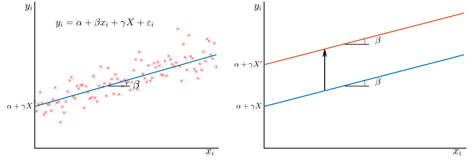
Scaling up the cross-sectional estimates is the equivalent to moving from one point to another on the line Panel A. But if there was a shift in aggregate government spending, the line would actually shift, as in Panel B. As a result, the aggregate effect is simply not identified from cross-sectional variation without additional assumptions. This is akin to the well-known microeconometric problem that age-, time-, and cohort-effects are not separately identified.

If you want to read about this more, you can check out Benjamin Moll’s slides, which highlight further examples of the missing intercept problem, and also explain why this issue is related to but different from the well-known ‘Reflection Problem’ (Manski 1993).

How can this problem be solved?

A simple short-term fix for economists

Put simply, whatever you do, please do not just scale up your micro-regression coefficients to the aggregate level. Authors should stop including such estimates, reviewers should stop asking for them, and journalists should stop cherry-picking them.

It is natural to want a simple, aggregate estimate of how X affects Y, that jumps off the page and puts results in a national perspective. However, it undermines the publication process when there is an incredibly high bar for causal estimates at a micro level, but a very low bar for considering how these effects scale to the aggregate. While quicker and easier, it’s bad for economics that many of the ‘facts’ that travel the furthest, through journalists looking for a good headline, or those who post abstracts with one-line takeaways on social media, are based on extremely strong assumptions that are unlikely to ever be satisfied – i.e. are inaccurate.

Longer-term solutions

To recover the missing intercept, and more accurately estimate aggregate impacts, research requires more structure. Long story short, this means a model. Not necessarily a full structural model, but a 'model' in the sense of assumptions that impose additional structure on the causal relationship between variables. There are different strategies for achieving this:

• Using full-blown structural macro models to convert regional estimates into partial and general equilibrium effects. For example, Mushfiq Mobarak joined the VoxDev podcast to discuss how rural-urban migration impacts welfare in the developing world. This research combined a general equilibrium model with the results of a field experiment that subsidised seasonal migration. Another well-known paper is Nakamura and Steinsson (2014), which estimates the impacts of government spending in the US.
• Using a bit of structure plus macroeconometric estimates from aggregate variation. In rare cases, credible identification of certain aggregate effects is possible from aggregate data, typically exploiting time-series variation. These macroeconometric estimates can then be combined with the microeconometric, cross-sectional estimates to answer the question of interest. For example, Wolf (2023) combines time-series evidence on military spending multipliers with cross-sectional estimates of consumption responses to fiscal stimulus checks to get at the aggregate effects of such stimulus under a ‘demand equivalence’ assumption.

Essentially, the missing-intercept problem would benefit from greater collaboration between micro- and macro-economists. This type of cross-silo work is exactly what STEG looks to foster.

References

The Missing Intercept: A Demand Equivalence Approach Christian K. Wolf American Economic Review vol. 113, no. 8, August 2023 (pp. 2232–69)

Fiscal Stimulus in a Monetary Union: Evidence from US Regions Emi Nakamura Jón Steinsson American Economic Review vol. 104, no. 3, March 2014 (pp. 753–92)

What Do We Learn from Cross-Regional Empirical Estimates in Macroeconomics? Adam Guren, Alisdair McKay, Emi Nakamura, and Jón Steinsson NBER Macroeconomics Annual Volume 35 2020

Regional data in macroeconomics: Some advice for practitioners Gabriel Chodorow-Reich Journal of Economic Dynamics and Control Volume 115, June 2020, 103875

Identification of Endogenous Social Effects: The Reflection Problem Charles F. Manski The Review of Economic Studies, Volume 60, Issue 3, July 1993, Pages 531–542, https://doi.org/10.2307/2298123