


Valuing the time of the self-employed is crucial for evaluating interventions and conducting cost-benefit analysis. Yet research often misprices this value at zero or equal to market wages. New evidence from Kenya suggests a practical fix: value unpaid self-employed labour at 60% of the local market wage.
Editor's note: The authors have made slides available to accompany this research here.
Many development programmes change how people use their time: a new technology may enable farmers to spend less time irrigating, or micro-entrepreneurs more time on bookkeeping. However, for one significant category of workers – the self‑employed – changes in time use are not directly priced by the market because they are not paid a wage. Even when similar jobs exist – say, casual workers performing farming tasks – their wages can misprice unpaid labour when markets are incomplete (Benjamin 1992, LaFave and Thomas 2016, Breza et al. 2021). How should policymakers value interventions that change farm or business revenue while also changing hours worked?
Correctly valuing the time of the self-employed is essential for estimating the welfare impacts of policy and conducting cost-benefit analyses. Since many new technologies require more of users’ time, ignoring time costs can make these technologies appear more profitable than they are (Suri 2011). The difficulties in valuing time have left many researchers to rely on crude assumptions or attempt to bypass the issue altogether – estimating only revenue, instead of profits, for instance. In a recent review of recent development papers, we find that the majority valued self‑employed time at zero, while a minority use the market wage or demonstrate sensitivity to different assumptions about the value of time.
Figure 1: How the literature values self-employed time in low-income countries
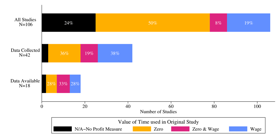
Notes: Most papers either ignore the cost of self‑employed labour or set it to zero; far fewer use market wages or explore ranges. We analysed N=106 studies of the self-employed measuring profit or revenue impacts. Of these, N=42 collected the data needed to account for the value of time, and we were able to obtain that data from N=18.
A new approach to measuring the value of time
In recent research (Agness, Baseler, Chassang, Dupas, and Snowberg 2025), we worked with smallholder households in Kenya and offered them trades between money, time, and a good (a lottery for an irrigation pump). Each participant completed three incentivised choices: (i) performing two hours of casual farm work for a cash wage, (ii) paying cash for the lottery ticket, and (iii) performing casual farm work for the same ticket. From these, we compute two values of time: a direct value (cash-for-time) and an indirect value (willingness to pay in cash and time for the same good). If preferences are standard – even with credit limits or labour rationing – the two measures should coincide. We find that they do not.
Figure 2: Direct versus indirect value of time
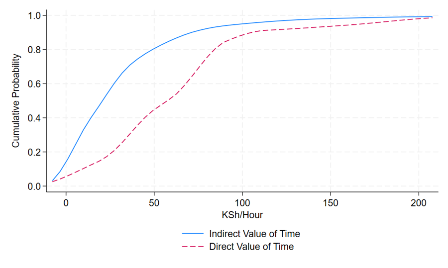
Note: For most people, the direct measure (cash‑for‑time) is much higher.
These two measures of the value of time are very different, but is either correct? We fit a structural model that allows for distortions (‘wedges’) in each exchange (cash‑for‑time, cash‑for‑good, time‑for‑good), which together produce the overall wedge between the direct and indirect values. By looking at how the overall wedge correlates with each of the three decisions, we can estimate the size of each individual wedge. Interestingly, the data points to wedges that arise only when participants trade cash; time-for-good decisions appear undistorted. Cash‑specific behavioural responses, such as loss aversion, are a parsimonious interpretation, but our method can be applied regardless of the source of the wedges.
The value of time for the self-employed
The value of time we compute from our model – the ‘structural’ value of time – is welfare relevant for many real production decisions. This estimate is around 60% of the average local wage for casual farm work and is stable across demographic and economic subgroups in our data. Even without modelling, our two empirical measures offer bounds: roughly 40–100% of the local wage. While this value is inherently context dependent, we offer suggestions to researchers and policymakers for estimation in different settings.
The cost of ‘mispricing’ time
If we value self‑employed time at zero, we will oversell time‑intensive technologies and undersell labour-saving ones. Applying the 60% rule (and showing 40–100% bounds) is straightforward and often flips conclusions, as demonstrated in Figure 3. Interventions that significantly change time use such as irrigation, genetically modified seeds, childhood health programmes, and index insurance are especially sensitive to value-of-time assumptions. For programmes that do not change labour supply much – such as sobriety incentives – valuing time correctly is less important.
Figure 3: Sensitivity of estimated impacts to the value of time
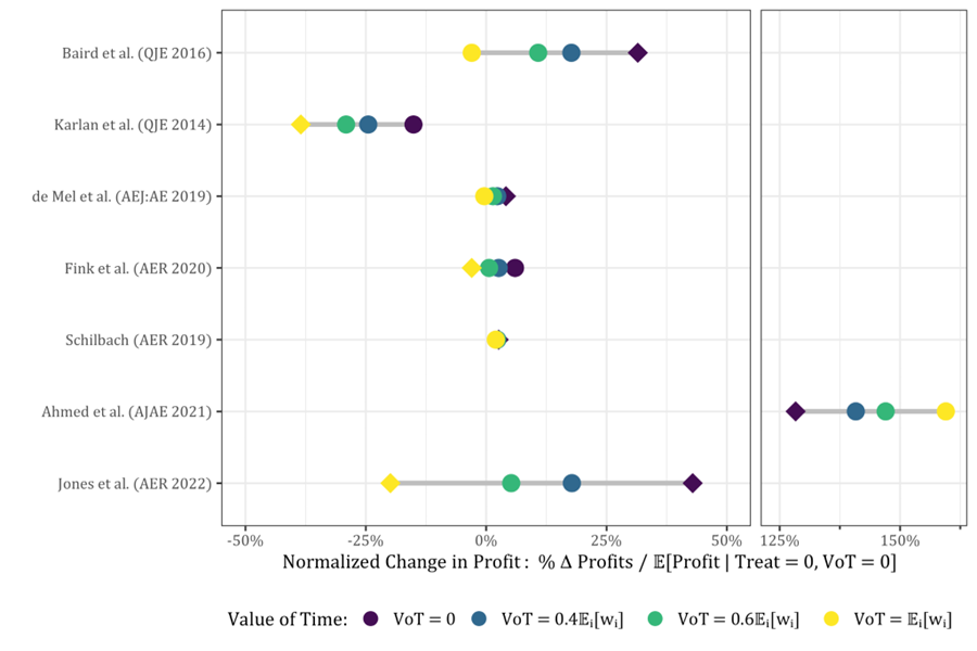
Notes: Normalised profit impacts for selected studies under 0%, 40%, 60%, and 100% of the casual wage (diamonds mark the value used by original authors).
How to use this in practice
We make the following practical recommendations:
- If an intervention changes how much time self‑employed people spend working, consider valuing that time at approximately 60% of the local wage.
- Concerned your setting differs? Two survey questions can help clarify: ask about the respondent’s recent casual wage and what they believe they could earn tomorrow. In places where jobs are more tightly rationed, the structural value of time is likely to fall further below the market wage.
- Which local wage should you use? Pick an activity as close as possible to the type of work your intervention affected: for example, casual farm labour if your programme changed work time on the farm. Keep in mind that work that can be scheduled flexibly will be less costly than work that must occur at a specific time.
- Consider whether the additional work time should be valued with or without the distortion that appears in our direct measure. Our data shows that time-for-good decisions, such as working longer for greater yield, are undistorted. But we also believe that naturalistic choices, such as a micro-entrepreneur working longer hours for more revenue, are unlikely to be distorted. If you are unsure, apply the 40–100% bounds described above.
- Because our method uses linear approximation, it should be applied with caution (and ideally show bounds), especially if your programme significantly alters work time.
- Running a big study that requires precision? Replicate the three short, incentivised elicitations on a subsample; identification relies on the joint pattern across the three choices.
Implications for labour policy on self-employment
We make the following policy recommendations:
- Do not treat unpaid work time as free. At a minimum, use 60% of wage as your default; show 40–100% bounds.
- Expect conclusions to change. Time‑intensive programmes will look less attractive; labour-saving ones more so.
- Measure work time. Even if you elicit accounting profits directly, record self‑employed hours so profits can be adjusted for time.
- Design for time. Interventions that save scheduling pain or reduce peak‑time work may deliver large welfare gains beyond output.
References
Agness, D, T Baseler, S Chassang, P Dupas, and E Snowberg (2025), “Valuing the time of the self-employed,” Review of Economic Studies, rdaf003.
Ahmed, A U, J Hoddinott, N Abedin, and N Hossain (2021), “The impacts of GM foods: Results from a randomized controlled trial of Bt eggplant in Bangladesh,” American Journal of Agricultural Economics 103(4): 1186–1206.
Baird, S, J H Hicks, M Kremer, and E Miguel (2016), “Worms at work: Long-run impacts of a child health investment,” Quarterly Journal of Economics 131(4): 1637–1680.
Benjamin, D (1992), “Household composition, labor markets, and labor demand: Testing for separation in agricultural household models,” Econometrica 60(2): 287–322.
Breza, E, S Kaur, and Y Shamdasani (2021), “Labor rationing,” American Economic Review 111(10): 3184–3224.
de Mel, S, D McKenzie, and C Woodruff (2019), “Labor drops: Experimental evidence on the return to additional labor in microenterprises,” American Economic Journal: Applied Economics 11(1): 202–235.
Fink, G, B K Jack, and F Masiye (2020), “Seasonal liquidity, rural labor markets, and agricultural production,” American Economic Review 110(11): 3351–3392.
Jones, M, F Kondylis, J Loeser, and J Magruder (2022), “Factor market failures and the adoption of irrigation in Rwanda,” American Economic Review 112(7): 2316–2352.
Karlan, D, R Osei, I Osei-Akoto, and C Udry (2014), “Agricultural decisions after relaxing credit and risk constraints,” Quarterly Journal of Economics 129(2): 597–652.
LaFave, D, and D Thomas (2016), “Farms, families, and markets: New evidence on completeness of markets in agricultural settings,” Econometrica 84(5): 1917–1960.
Schilbach, F (2019), “Alcohol and self-control: A field experiment in India,” American Economic Review 109(4): 1290–1322.
Suri, T (2011), “Selection and comparative advantage in technology adoption,” Econometrica 79(1): 159–209.